CUSUM

CUSUM: Using Quality Control Method to Remove Random Noise

This page discusses my attempt at smoothing out a noisy signal, using the CUSUM method.

CUSUM (Cumulative Sum of Departure from a standard) was developed by Page from Cambridge in the mid fifties as a method of quality control, to detect drifts in the data

The idea is that, if you progressively add the differences between each measurement and a standard, the random noise would cancel each other out, and any persistent departure from the standard will accumulate and gradually become aparent.

The problem was that, as data are accumulated, the mean gradually increases. This made the method difficult to used, as the values have to be plotted, and visually compared with a mask containing decision borders.

In the mid eighties, Hawkin and Olwell, from Minnesota, developed a correction factor called reference factor (k), and did away with the need for masks and visual inspections. The method was then widely adopted in industry, to detect small defects early.

In the late nineties, when I was running the hospitals, I adapted the method to detect drifts in patient satisfaction, and found that it was both sensitive and easy to use.

I have decided therefore just to try it and see if it can be used.

CUSUM Explained

The complexities of CUSUM are mostly related to its adaptation to different numerical distributions and to estimate probabilties, so that a reliable decision can be made that the departure from the stadard is significant enough to raise an alarm and call to action.

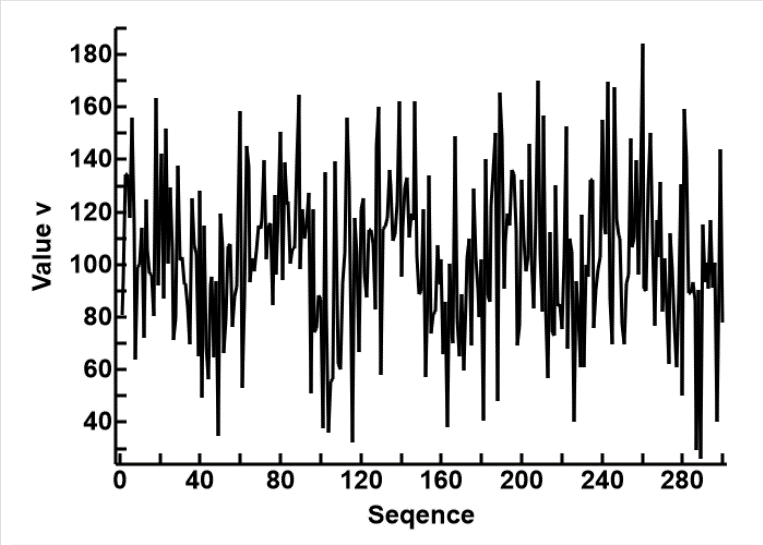
For our purpose, where we are using the method to smooth out irregularities in the data, and when our data contains only linear measurements (perhaps normally distributed), the technology is simple.

If the normal value is N and abnormal value is A, then the reference factor is k = (A + N) / 2
In a series of continuous measurements, the current CUSUM value is the previous one, plus the difference and subtracting the reference factor
C_i = C_i-1 + V_i - r, where V_i is the current value
If C_i crosses the standard value N, then it is defaulted to N
After being used for correction of the next data point, the CUSUM is corrected by subtracting the standard value to produce the final value C_i,final = C_i - N
For quality control purposes, usually only one CUSUM is calculated, detecting departure in the direction of interest
In order to adapt the method for our use, 2 CUSUM, for departure in both directions, can be used

The First Try

The 4 plots to the right demonstrated my first try, just to see if the method is potentially useful.

The first plot shows the input data, Noise_3
The second plot shows the two CUSUM obtained, one for departure upwards, the other downwards. The parameters used are
- For Noise_3, The mean μ = 100, and this is used as the sstandard or normal N=100
- The departure assigned is 2, so A_up=102, and A_down=98
The third plot combined the two, for any data point C = C_up + C_down
It can be seen that a fairly clean set of curves now appear, and all but one overlap value (near the right end) have been resolved
The fourth and last plot superimposed the CUSUM plot onto the Noise_3 plot, to demonstrate their relationship. Please note
- The black lines represnt Noise_3. The lines are thickeded to form the background
- The red line is CUSUM. Note CUSUM is cumulative differences and not the same measurement as Noise_3. It is rescaled to fit in the same plot, to demonstrate time relationship
- As with any averaging processes, the is a phase lag, so that the peaks and troughs of CUSUM are a bit to the right of those from Noise_3

A more Extensive Exploration

"""
CalCUSUM is the engine

inputLst is the list of input data in SD units with mean=0 and SD=1
zDiff is the difference to detect also in SD units
  - reference factor k = zDiff / 2
  - 2 separate CUSUMs are calculated, for upward and downward departures 
"""
def CalCUSUM(inputLst, zDiff):
    k = zDiff / 2         # reference factor
    baseVal = 0           # mwan= 0 SD=1
    kk = -k               # for the opposite direction
    cusumA = [baseVal,baseVal]            # results
    cusum = [baseVal*2,baseVal*2]         # calculations
    resLsts = [[0] * 2 for i in range(len(inputLst))] # resul to be returned
    oldCusum = cusum;
    for i in range(len(inputLst)):
        v = inputLst[i]                    # each value
        cusum[0] = oldCusum[0] + v - k;    # current CUSUM
        cusumA[0] = cusum[0] - baseVal;    # correct for baseline
        if cusumA[0]baseVal:
            cusumA[1] = baseVal
            cusum[1] = baseVal * 2
        resLsts[i][0] = cusumA[0]
        resLsts[i][1] = cusumA[1]
        oldCusum = cusum;
    return resLsts                       # return results as 2 column list

"""
Main controlling function for CUSUM
  - reads in from file
  - extracts the correct column
  - convert into z=(v-mean)/SD
  - call calculations
  - append the 2 result lists (up and down) to data
  - sata to csv file
"""    
def TestCUSUM():
    datLsts = TextFileToLists("InputNoise_3.csv")
    cols = len(datLsts[0]) 
    inputLst = GetColFromLists(datLsts,4)      # Noise_3 as text+label
    del(inputLst[0])                           # remove label
    inputLst = StrListToFloatList(inputLst)    # Noise_3 as numbers
    mean = statistics.mean(inputLst)
    sd = statistics.stdev(inputLst)
    datLst = []                                # turn to z=(v-mean)/SD
    for v in inputLst:
        datLst.append((v-mean)/sd)
        
    for i in range(5):                        # do 5 times at 0.1 intervals
        zDiff = 0.1*(i+1) # SD from mean
        outputLsts = CalCUSUM(datLst, zDiff) # call calculation

        tmpLst = GetColFromLists(outputLsts,0)        # upwards result
        tmpLst = NumListToFormatList(tmpLst, "{:.4f}") # results as str
        InsertIntoList(tmpLst, 0, "Pos" + str(zDiff))  #label
        datLsts = InsertColumnToLists(datLsts, cols, tmpLst) #append to data
        cols += 1
        tmpLst = GetColFromLists(outputLsts,1)       # same for downward res
        tmpLst = NumListToFormatList(tmpLst, "{:.4f}") 
        InsertIntoList(tmpLst, 0, "Neg" + str(zDiff))
        datLsts = InsertColumnToLists(datLsts, cols, tmpLst)
        cols += 1
    ListsToFile(datLsts, "CUSUM.csv")

As the method looks promising at this initial stage, I have placed the program I develped (see panel to the right) for you to look at. It is rather long winded as I was focussed on explanation and not efficiency.

Also, as the results from CUSUM analysis is the departure from a baseline, there is no longer any need to stick to any unit of measurement. I have therefore use the z unit (z = (v-mean) / SD), so all the results have a mean of 0 and SD of 1.

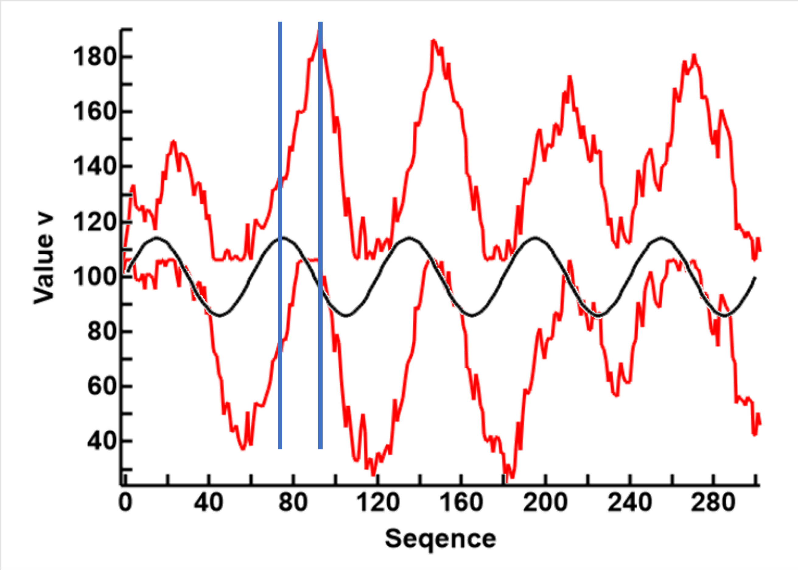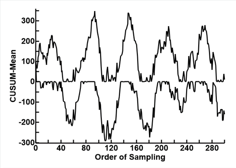
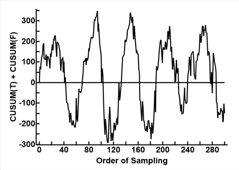
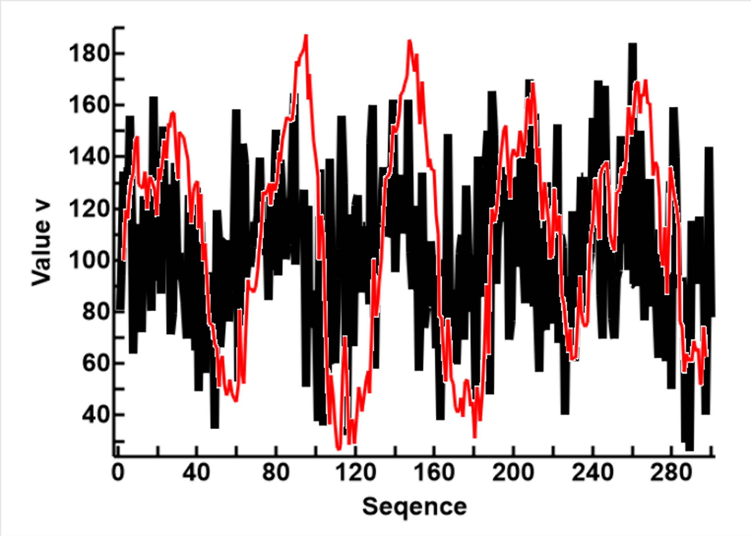
The first thing I noticed is a very obvious phase shift, as seen in the first plot on the left. This is much more pronounced than any of the averaging methids used befire. This matters if we are to integrate CUSUM with any other processes mathematically, as the phases must be aligned

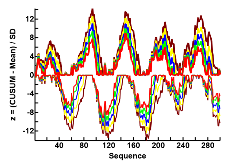
I then tested the effects of using diferent reference factors (k) on the shape and size of the CUSUM results, the results are shown in the second plot to the left. Having scaled the measurements to mean=0 and SD=1.
  -Maroon: zDiff=0.1, k=0.05
  -Yellow: zDiff=0.2, k=0.1
  -blue: zDiff=0.3, k=0.15
  -green: zDiff=0.4, k=0.2
  -red: zDiff=0.5, k=0.25

It can be seen that, as the reference factor (k) increases, the CUSUM curve becomes smaller and smoother.

With a k value high enough, the curves are plattened out altogether, and the CUSM line becomes a trend line,

At this stage, the k value is chosen by trial and error. However, I suspect the idel k value can be calculated, based on the width and amplitude of the curve, and the level of moise.

One advantage is therefore that the method can be used flexibly, tweaked to suit the purpose at hand

Comments and Opinions

I have been pleasantly surprised to see how well this method works, but to use it, there is a need to test it extensively. It works well at this initial test, because the noise is random, evenly distributed, and able to cancel itself out. How the text behaves if the noise has changing patterns of frequency and amplitude requires extensive testing. It is also unclear at this stage how the method will work if the signal is a compound one, a combination of multiple waves.

As I am now keen to proceed into splitting the signal into bipolar conclusions of true/false, I will not proceed to test this method extensively until I have some feedback from you