 The solution is as follows, using the plot to the left to demonstrate
 This page addresses transformation of a linear measurement into that with probabilistic distribution
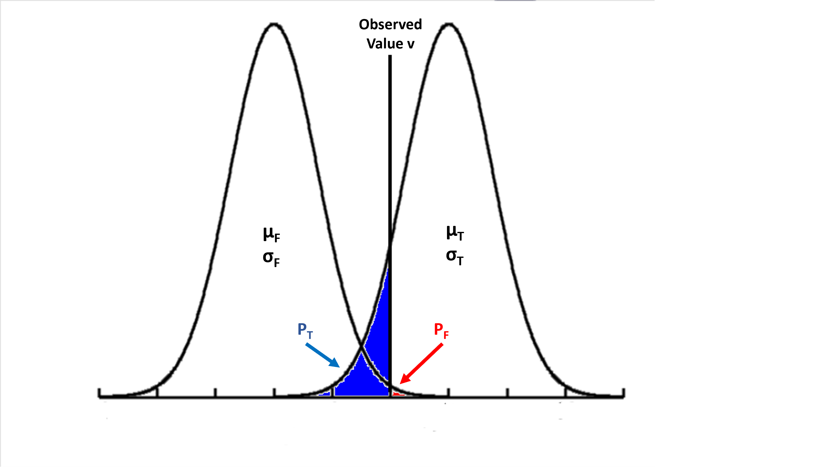
It began with a simple question, represented by the plot to the left, that With two groups of normally distributed data
Group true (T) with mean μT, SD σT
Group false (F) with mean μF, SD σF
What is the probability of any value v belonging to either groups.
The solution is as follows, using the plot to the left to demonstrate
The red area is the proportion of group F define by the value v (PF)
The blue area is the proportion of group T defined by the value v (PT)
The ratio of these 2 proportion is an odd O, OT = (PT) / (PF)
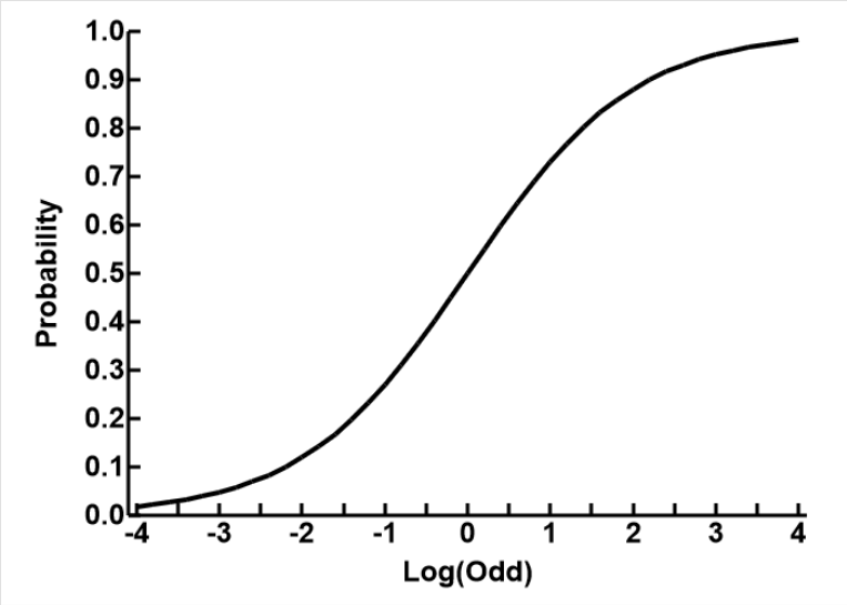
The relationship between odd and probability π is
π = 1 / (1 + exp(-O))
as shown in the plot to the right
The area P for any normal distribution can be calculated as follows
Distance from the mean in SDs z = abs(μ - v) / σ
The probabbility P can be obtained by the Python function P = scipy.stats.norm.cdf(1 - z)
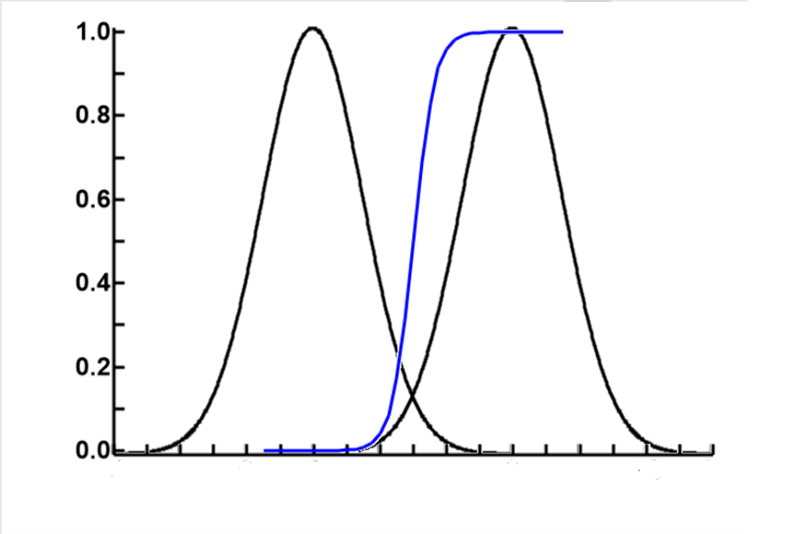
The results of these calculations are as shown in the blue line in the plot to the left. Please note that the vertical axis is scaled to probability and not to the height of the two normal distributions. The 2 normal distribution curves are there to show the relationship between probability and the horizontal values
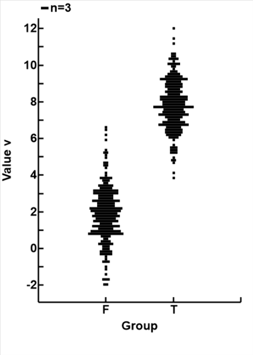
The plot below and to the left shows how well the theory described so far is reflected in that data.
The theoretical relationship between value v and probability of being in group T πT is shown by the blue line. This line is calculated based on the parameters that the two means are μT=2 and μT=8, and both groups have the same SD σ=1.5
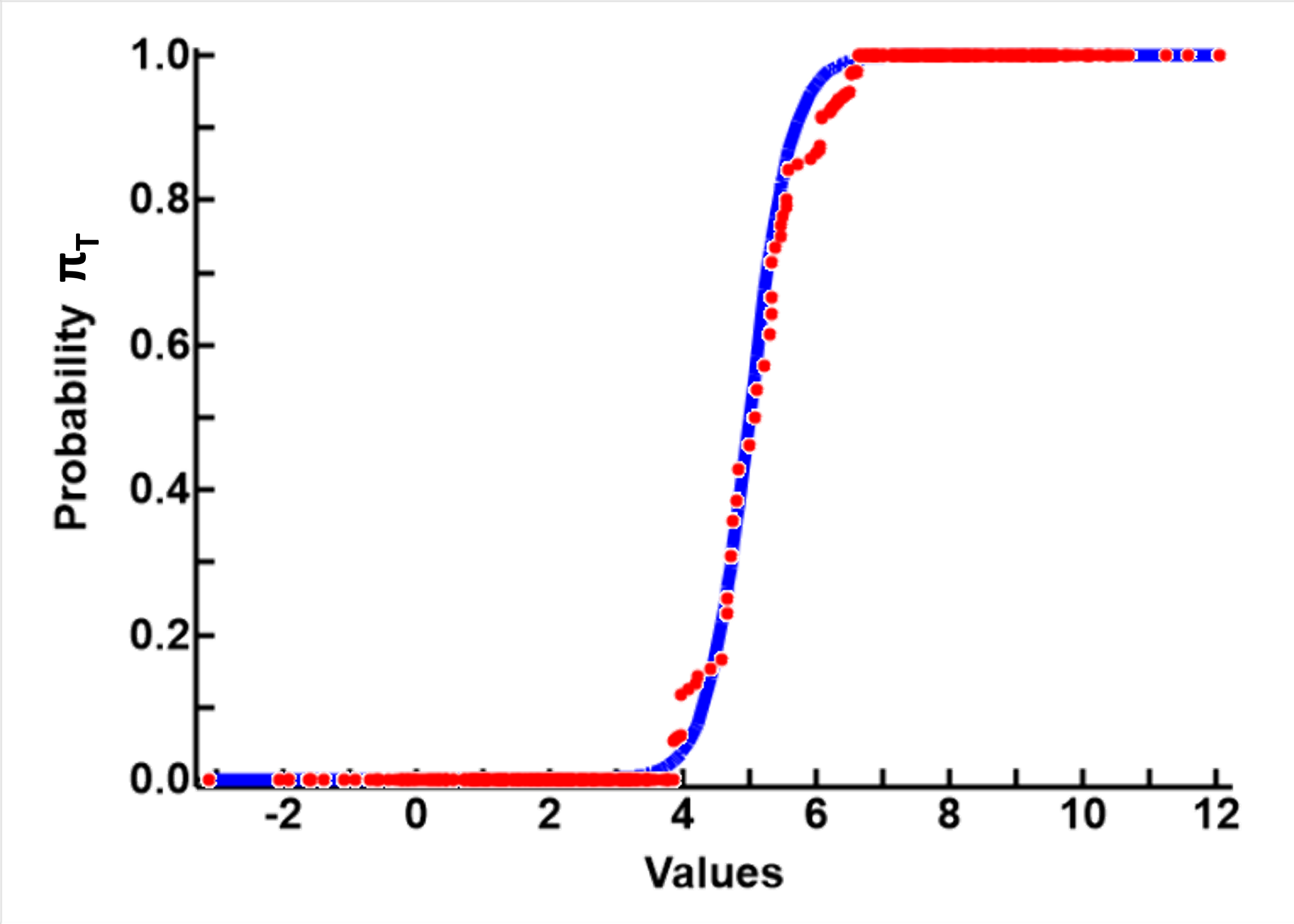
The probability of the value in each data point is shown as the red circle.
This plot demonstrates that, other than minor discrepencies caused by random variations in the computer generated data, the theory and the mathematics seem valid
![]() Additionally, this algorithm provides a mean of transforming data from a Gaussian distribution to a probabalistic one. As probabilistic distributions compresses intervals near the extremes and expands those in the middle, it can be used to enhance the separation data values between the two groups.
Additionally, this algorithm provides a mean of transforming data from a Gaussian distribution to a probabalistic one. As probabilistic distributions compresses intervals near the extremes and expands those in the middle, it can be used to enhance the separation data values between the two groups.
This can be demonstrated in the plot to the right, using the same testing data. The algorithm compresses all non-overlapping values to 0 and 1, and the overlapping values as probabilities of belonging to group T (πT)