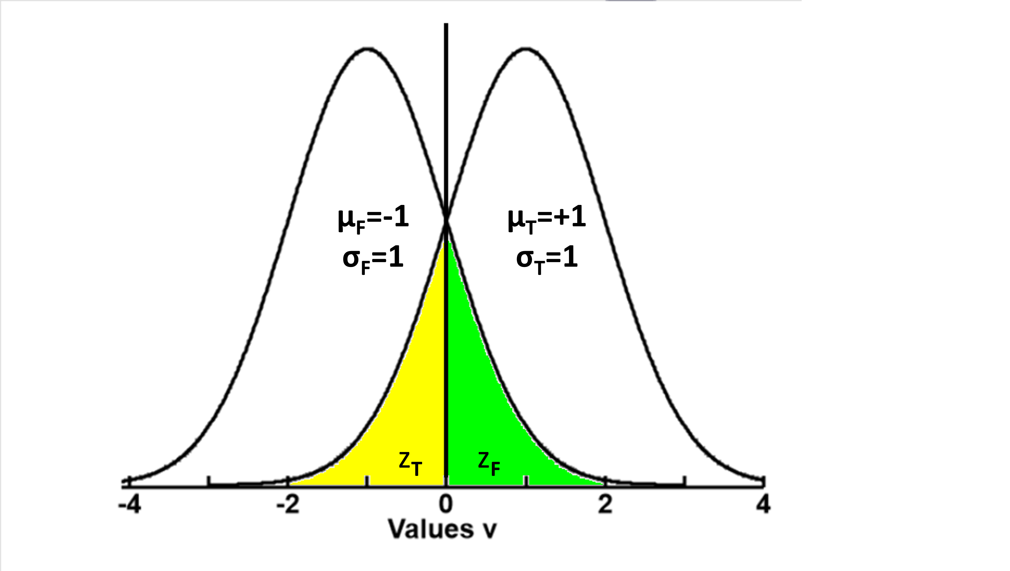
 The situation is as shown in the plot to the left. There are two groups (false F and true T) of measurements that have a common Standard Deviations (σ), but different means (μF, μT). The question is, what is the proportion of total data that have overlapping values.
To demonstrate the calculations, we will use a common SD σ=1, and the mean of group false μF=-1, and mean of group true μF=+1t
The calculation is as follow
- The two normal curves meet at midpoint between the two means (μT - μF), where the value v=0
- The green area represents the probability of overlap from group false (αF), where data from group F have lower values. zF = (v - μF) / σ = 1
- The yellow area represents the probability of overlap from group true (αT), where data from group T have higher values. zT = (μT - v) / σ = 1
- The area under the normal distribution curve outside of z=1 is α=0.16. Values of α for any z can be obtained using function norm.cdf(z) in the Python package of scipy.stats
- The probability of overlap is then (αF + αT) / (1 + 1) = α = 0.16 (16%)
- Putting all this together, Probability of overlap P = norm.cdf(((μT - μF) / 2) / σ)
| N(no overlap)/N(overlap) | z = (μT - μF) / σ |
| 101 | 2.5631 |
| 102 | 4.6527 |
| 103 | 6.1805 |
| 104 | 7.4380 |
| 105 | 8.5298 |
| 106 | 9.5068 |
| 107 | 10.3987 |
| 108 | 11.2240 |
| 109 | 11.9956 |
| 1010 | 12.7227 |
| 1011 | 13.4120 |
| 1012 | 14.06897 |
| 1013 | 14.6975 |
| 1014 | 15.3015 |
| 1015 | 15.8829 |
| 1016 | 16.4191 |
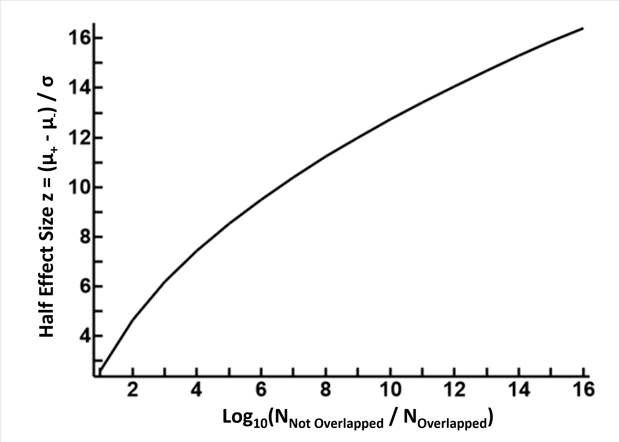
The plot to the left and table to the right demonstrate this relationship. Please note that, the table and plot refer to the effect size which is (μT - μF) / σ, not half of this value used during calculations
Opinion and Comments
In reference to the current calculations, to have an overlap rate of less than 1 in a million (106) will require the difference between the two means to be 9.5 SDs or more. It is therefore unrealistic to hope that increasing precisions in the machinery can prevent data from overlapping. Given the nature of normally distributed measurements, overlap is inevitable, so the focus should not be on how to avoid it, but on how to deal with it.
More generally, I am reminded that, during our conversation in Cambridge, we used the term probability to mean different things, and this caused some confusion. If we are to have a continued conversation in statistics for engineering, I think we should clarify how this term is used. I shall provide an actual incident to demonstrate this.
There is a heart defect in newborn babies that is inevitably fatal, but operation to repair this defect is dangerous. Over the years, after a lot of data collection and international discussion, it was accepted by everyone that the death rate for the operation should be around 14%.
One of the hospital in Hong Kong appointed a new heart surgeon, and in his first 8 operations for this heart condition, 5 died (62.5%). When other doctors in the hospital became alarmed the heart surgeon protested that the numbers were too few to make a judgement. I was asked to help, and I used a well known statistics test the Binomial Test, which concluded that the Type I Error (the probability that 5 cases out of 8 is no different to 14%), is 0.0021, very unlikely. This allowed the conclusion that the death rate was too high, and a full investigation was launched. The surgeon was found to be a fake, a lot of qualifications were bought, and a lot of his stated experience were lies.
This case demonstrates the use of probability 3 ways
- The expected probability of 14% (0.14) reflects reality, gained from evidence of research and past experience
- The 5 out of 10 probability, 62.5% (0.625), is a description of proportion in a single instance
- The Type I Error, the probability that 5 out of 8 is not different to 14%, is a theoretical probability, based on many assumptions, that the patients and hospital conditions had acceptable standards, that the binomial distribution used in this calculation is close enough to the normal distribution, and there are no other causes for death in this cohort. This probability is merely a numerical expression of how confident we are about our conclusion.
To prevent my own confusion, I use the term proportion to represent observed or expected frequencies, abbreviated to P or p. For probabilities based on statistical modelling or representing level of confidence I use the abbreviations α and π. α was used by Fisher (father of mordern statistics) to represent Type I Error and this is universally accepted. π is used often in disussions about Bayesian probability, to separate observed and estimated probabilities.
During our conversation in Cambridge, you were talking about the expected frequency of overlapping observations, based on means and SDs in 2 normal distributions, and I think this is fallacious thinking. Mean and SD are estimated from data, and represents a description of what the observed values were, and that one cannot declare an absolute margin between what is and is not possible. It cannot be turned around and used to predict the frequency of occurences in an infinite range. For example, the mean and SD of the height in an adult human are, say, 5 and 1 feet (a guess for this conversation). According to normal distribution, the probability of having a 1 foot high man (5-1)/1 = 4SDs is 0.000032, 3 to 4 per 10,000. However, with more than 4 billion people on earth I have never seen or heard of a 1 foot man (height, not what you walk on), and I am pretty sure that he dos not exist