Smoothing Noisy signals
The initial Signal
This page discusses my varying attempts to smooth a sequence of signals. The Date used is as shown in the 3 plot to the right (see MakeData.html)
The sequence has 300 data points and contain the following
- It began as a sine wave with no noise, hence Noise_0 (n_0)
- The data points are 6 degrees (out of 360) apart. Each sine wave has 60 data point, 30 for each peak or trough
- The sine wave was rescaled to mean μn_0 = 100 and SD σn_0 = 10
- All values <=100 are classified as group false (F), all values >100 as true T
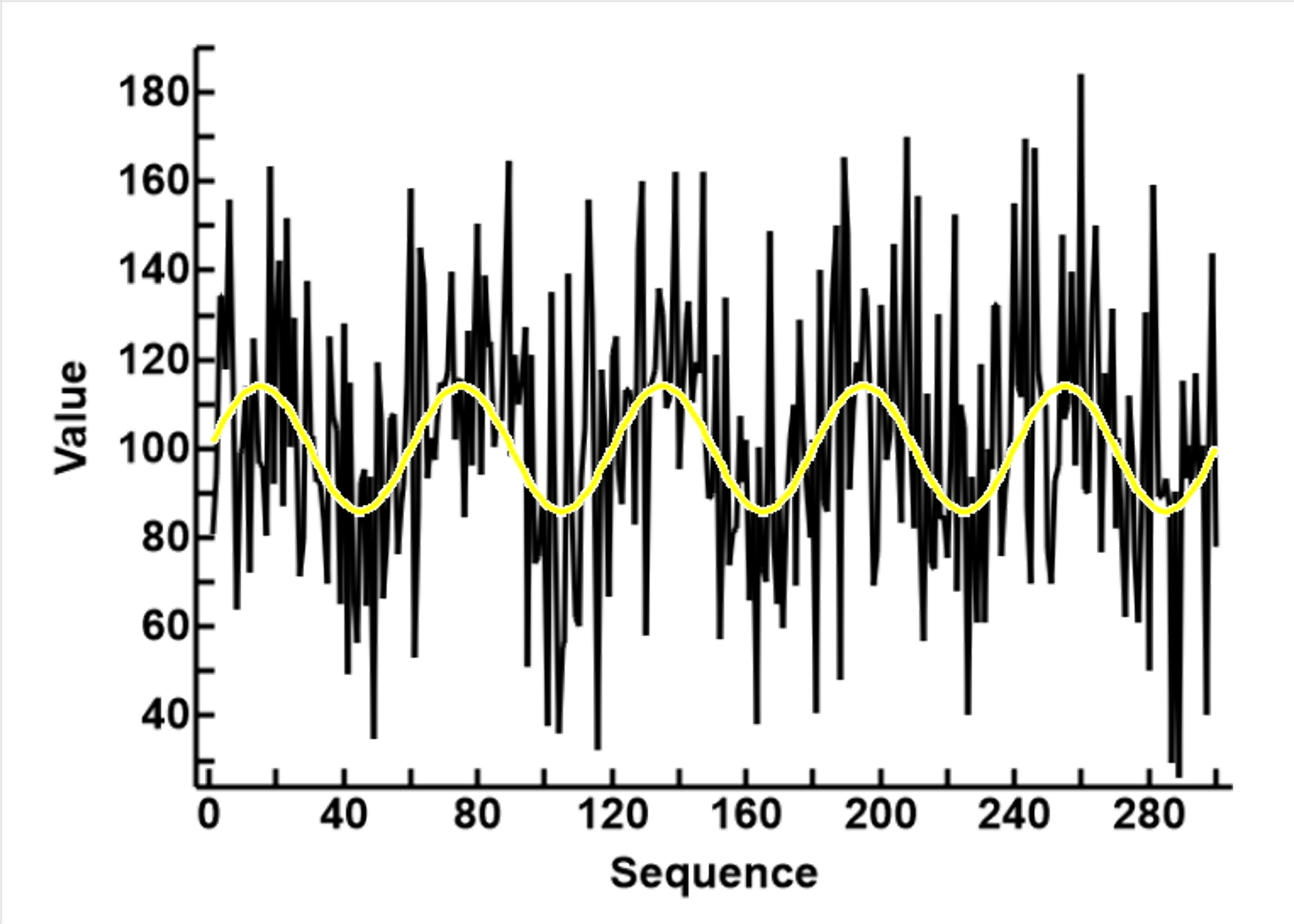
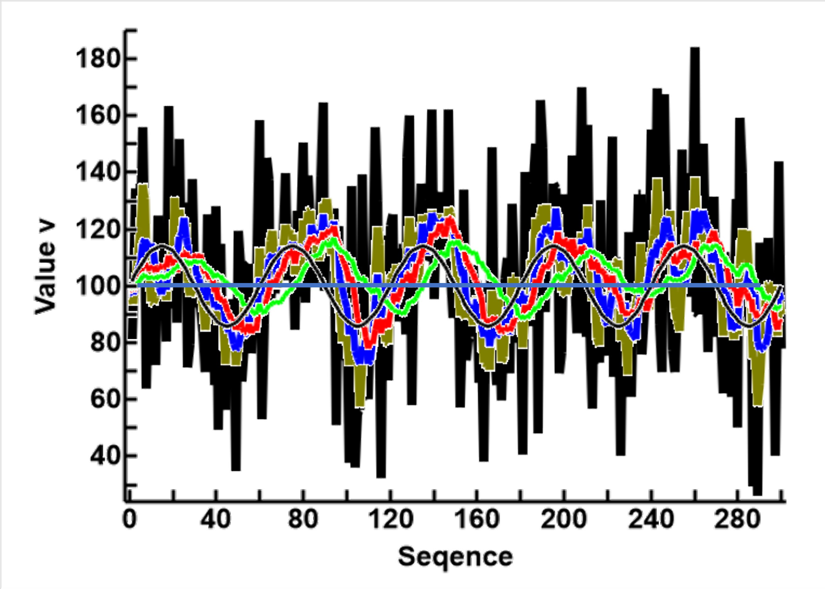
- Noise_0 is shown in the first plot to the right as the yellow line
- A noise is added to Noise_0.
- The noise is a set of randomly generated normally distributed value with mean 0 and SD of 30 (3 times that of Noise_0)
- Each noise value is added to the Noise_0 value, thus creating Noise_3 (n_3)
- Noise 3 is shown as the black line in the first plot to the right, and is used as the initial signal for the rest of this page
The addition of noise caused the distortion of Noise_1, these distortions are
- The amplitude is enlarged, as shown in the black and yellow lines in the first plot
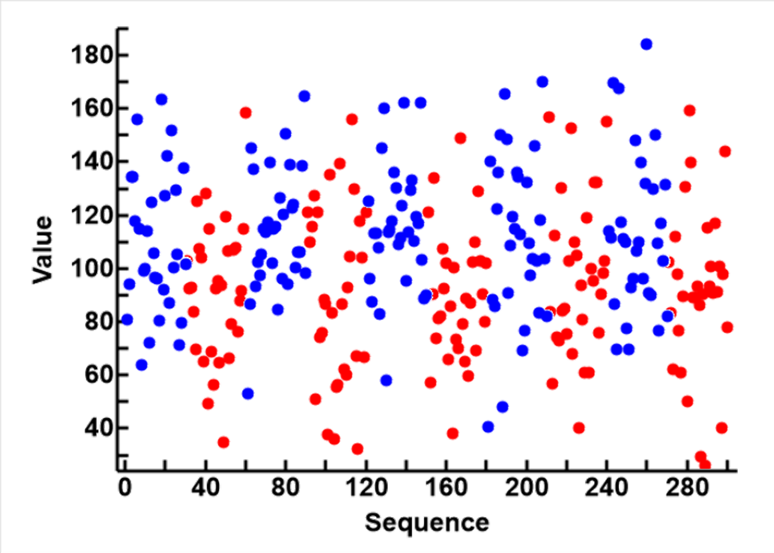
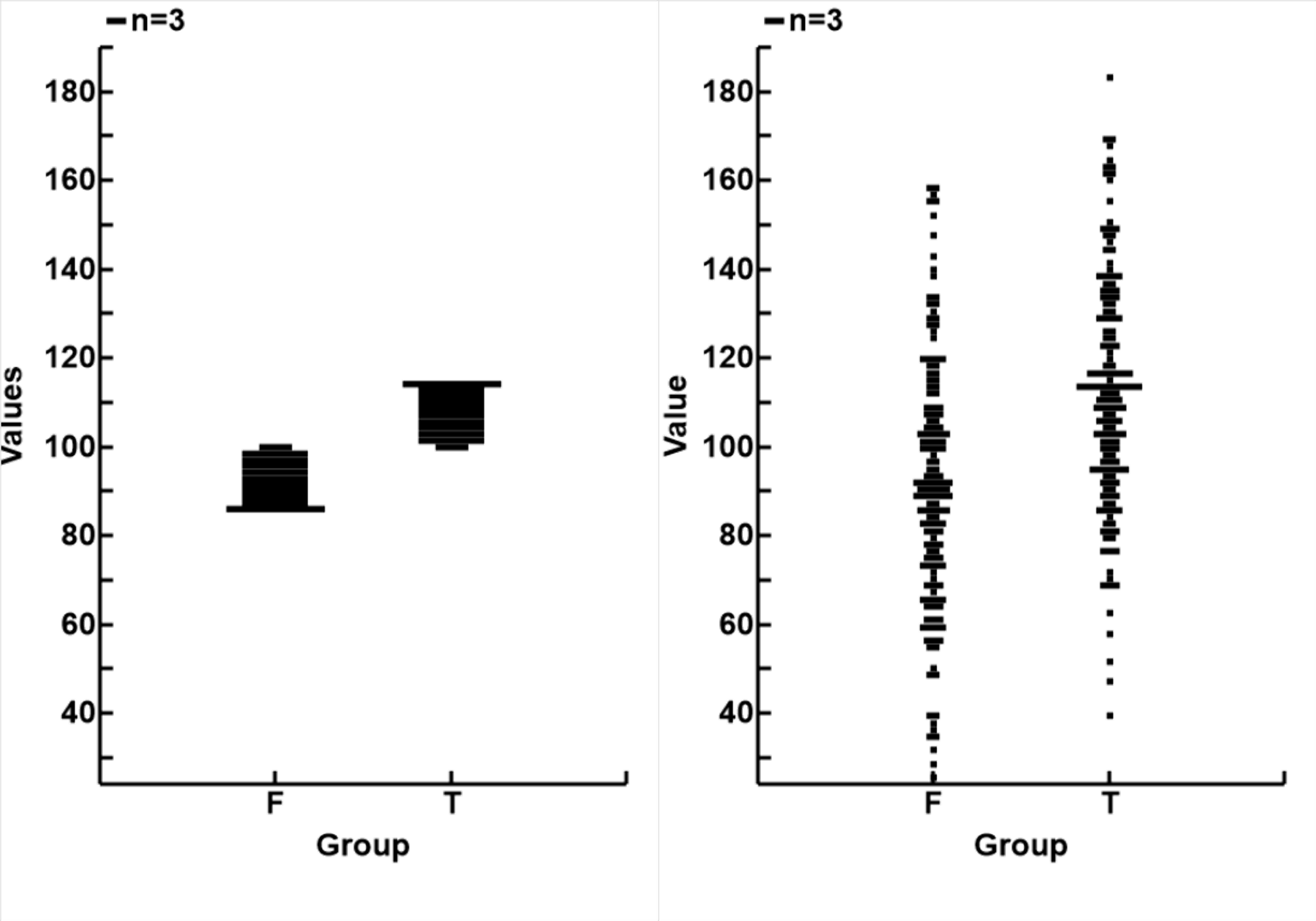
- There are considerable overlaps between the two groups (the peaks (T) and troughs (F) of Noise_0), as shown as the blue (T) and red (F) circles in the second plot, and the distributions of the two groups in the third plot. The distributions for Noise_0 to the left and Noise_3 to the right
| F | T | All |
| n | 150 | 150 | 300 |
| Noise_0 | |
| mean | 91.0201 | 108.9799 | 100 |
| SD | 4.3767 | 4.3767 | 10 |
| Noise_3 | |
| mean | 92.0824 | 112.5713 | 102.3268 |
| SD | 28.9289 | 26.8896 | 29.7096 |
The numerical descriptions of the data are in the table to the left. The overall mean remained unchanged, the Standard Deviations has increased. σn_0=10 and σn_3=29.7). The difference betwwn the means of T and F narrowed, μT-μF=18 for Noise_0 and 21 for Noise_3
The differences between Noise_3 and Noise_1 is a what this page will now address. Noise_3 will be used as the initial signal
|
The Simple Algorithm
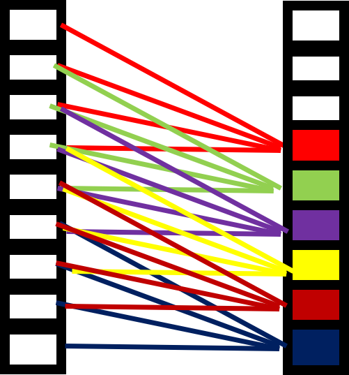
 The most obvious algorithm to use is the moving mean, where a moving window of sub-samples is used to create the mean value for each data point. The amount of averaging is controlled by the size of the window (WS). The diagram to the left represents this algorithm, using the current and previous 3 data points for averaging (WS=4)
Using Noise_3 as the initial data, the plot to the right shows the results of using this algorithm with different sizes. Please note that I used lines of different thickness so that the results from different runs so not onbscure each other on the plot. From the back to the front, in order of the window size, are
- The black thick line represents the inital data, Noise_3
- The teal color uses a window of 4 data points (WS=4, 0.07 of a wave, 0.13 of a peak or trough)
- The blue color uses a window of 8 data points (WS=8, 0.13 of a wave, 0.27 of a peak or trough)
- The red color uses a window of 16 data points (WS=16, 0.27 of a wave, 0.53 of a peak or trough)
- The green color uses a window of 32 data points (WS=32, 0.53 of a wave, 1.07 of a peak or trough). This is close to the original sine wave before noise was added(Noise_0)
- The thin black sinusoidal line represented Noise_0, when there is no noise
- The straight thin dark blue line shows the midpoint of the sine wave, where the value is 0
From these resullts, the following ideas are suggested
- Noise reduction is related to the size of the averaging window. This presents a potential granulation problem (the number of data points for a cycle of interest to that available for averaging)
- A window similar in size (number of data points) as the cycle of change is needed. This raises the potential for simultaneously using different size windows to focus on different waves, when the signal is a complex combination of multiple waves
- As the result of each calculation uses the current and a number of previous values, a phase shift, half the size of the window occurs. This presents an opportunity for error, if the results of multiple calculations, each with a different phase shift, were to be integrated
I will name this algorithm Simple Averaging
Addressing the Granulation Problem

 The frequency of events to detect and create are great in electronics, so that the time available to do so are small. The psossibility that the number of data points samples may be small compared with the with of the signal to be identified. There is therefore a need to consider whether analysis of similar quality as reported above can be achieved with very small window size
The smallest window size is two data points (WS=2). The question is whether using a 2 data point averaging repeatedly can achieve the same results as using a larger window. The scheme is presented to the left
The results of using the WS=2 repeated 8 times is compared with using average with a WS=8, and I shall call this algorithm Iterative Averaging.
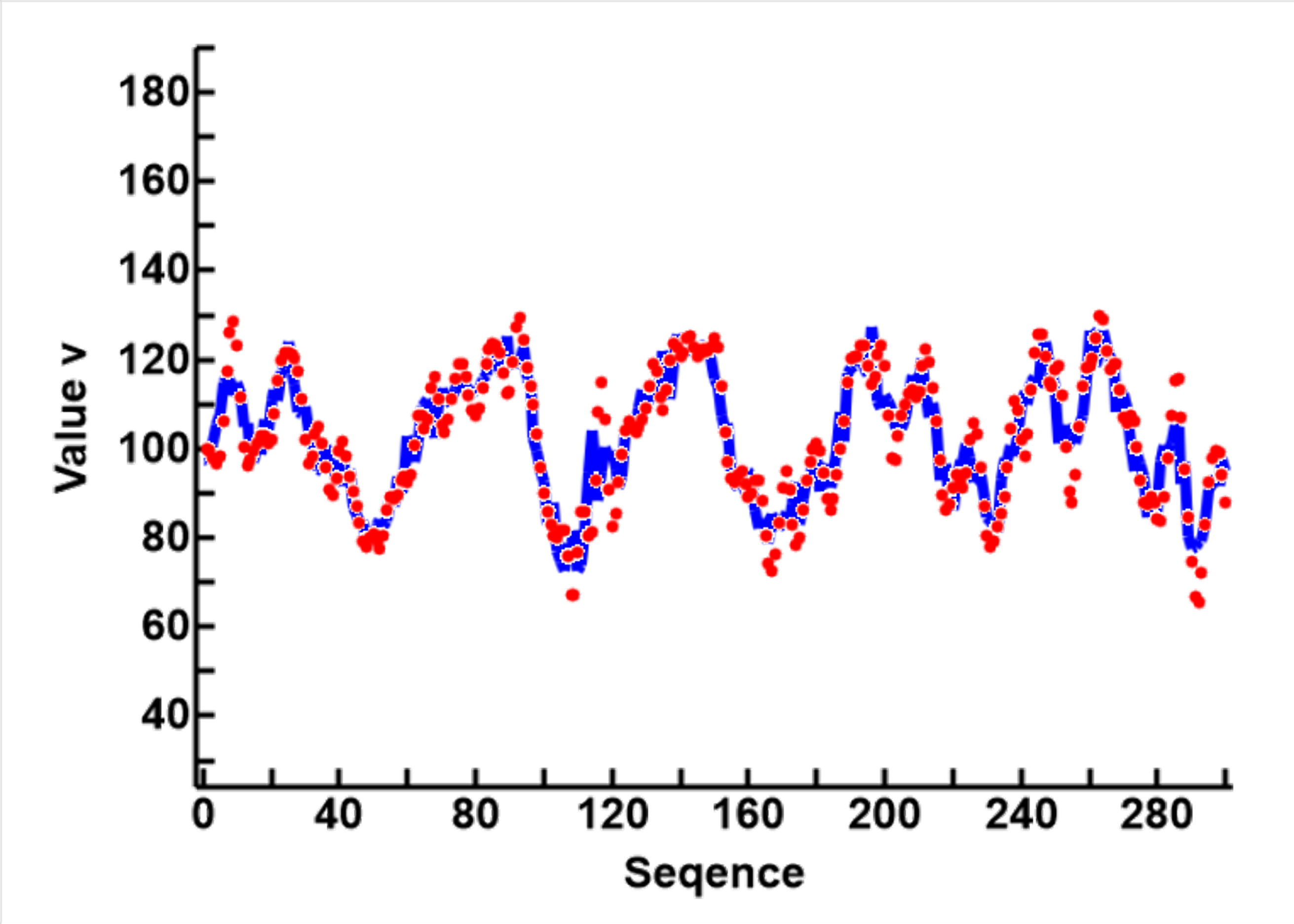
The results, compared with Simple averaging, are as shown in the plot to the right
- The blue line represents the results of Simple Averaging, using WS=8
- The red circles represent the results of Iterative Averaging, using WS=2, with the data recursed 8 times.
- Other than minor rounding errors, the results of the two approaches are almost identical
It can therefore be concluded that the granulation problem can be sidestepped by using Iterative Averaging, as it requires only 2 data points for calculations (WS=2). However, this requires iterative calculations, cannot be done in a single run, and therefore cannot be used in real time
The Single Run Algorithm
The small averaging windoe of WS=2 can be retained, and the iteration can be done in a single run, if each data point is iteratively everaged before the next data point.
In other words, the schema represented by the diageam above remains the same, but instead of doint the whole data set repeatedly, each single data point is repeated averaged before the next. I call this the Single Run Averaging
This will sidestep both the granulation problem, and with a single run, it can be adapted for real time calculations
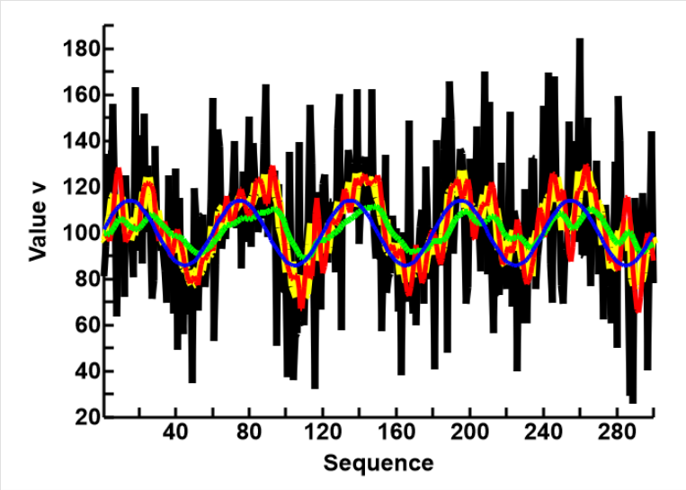 This was tried, and the results, compared with other algorithms are presented in the plot to the right
- The black line in the back represents Noise_3, the initial data
- The yellow line represents results from Simple Averaging, using 8 data points (WS=8), in a single run
- The red line represents results from Iterative Averaging, using 2 data points (WS=2), repeated 8 cycles
- The green line represents results from the Single Run Averaging, using an array of 8 windows, in a single run
- The blue line is the sine curve, Noise_0
As expected and reported earlier, the results from Simple and Itertive Averaging are almost identical.
I had expected the single Run Averaging to show similar results, but the results are very much better. Although the phase shift is the same as the other 2 methods, a much better smoothing effect was achived, and the amplitude was also smaller.
"""
inputList=list of input data, Noise_3
repeats=number of averaging, in this case 8
midlevel= mean or 0 in the sine curve, in this case 100
MakeListWith Constant creates the calculating array
    in this case a list of 8 cells, each with the value of 100
"""
def SingleSmooth(inputLst, repeats, midVal):
    refLst = MakeListWithConstant(repeats, midVal)
    resLsts = []
    for v in inputLst:
        resLst = [statistics.mean([refLst[0], v])]
        for j in range(1,repeats):
            resLst.append(statistics.mean([resLst[j-1],refLst[j]]))
            refLst[j] = resLst[j]
        resLsts.append(resLst)
    return resLsts
The interpretation is that One Run Averaging is more powerful, and can achieve greater smoothing with less resources, and causing less phase shift in the data. My real concern is that I do understand why this is so, and am worried that there is a mistake somewhere I had not seen.
I have therefore put the subroutine in Python code in the panel to the left for you to have a look at, and display the calculating data
 The results from Sngle Run Averaging, using WS=2, but arrays of 2 (blue), 4 (Yellow), 6 (red), and 8 (green) are shown in the plot to the right. Please note that I have expanded the vertical axis to separate the results for discussion.
It appears that the improvement with the Iterative Averaging is linear with increasing iteration, but logarithmic with One Run Averaging. Most of the smoothing are affected in the early cells, and after 4 cells further improvements are almost trivial
The advantage of this algorithms are therefore two fold
- Only very little resources are necessary
- The limits of smoothing can be found, at least by trial and error, and locked in for long term use
Comments and Opinions
I have made 3 attempts at using averaging to reduce noise in a data set. Although they sort of work, the results are not satisfactory.
My conclusion is that no form of averaging can reduce large amount of noise, especially when the signals overlap. This is only logical, as the overlapped data remain overlapped, no matter how the average is done.
On reflection, I think I have merely tried to re-invent the wheel. If mature engineers, with their truck loads of mathematical tools, have difficulties in this area, it is unlikely that I will make any significanct contribution.
I have therefore decided to abandon this direction of enquiry, and follow the statistical rather than mathematical approach